📝笔记：使用vlfeat的Matlab接口简单实现BOW以及VLAD

本文使用 vlfeat 的 Matlab 接口实现 BOW 以及 VLAD。另外，补充了有关NetVLAD的介绍。

BOW

BoW: Bag of Words，中译“词袋”，BoW算法即Bag of Words，本是用于文本检索，后被应用于图像检索，和SIFT等出色的局部特征描述符共同使用（所以有时也叫Bag of Feature，BOF），表现出比暴力匹配效率更高的图像检索效果，它是直接使用K-means对局部描述符进行聚类，获得一定数量的视觉单词，然后量化再统计词频或TF-IDF加权之后的权重系数。

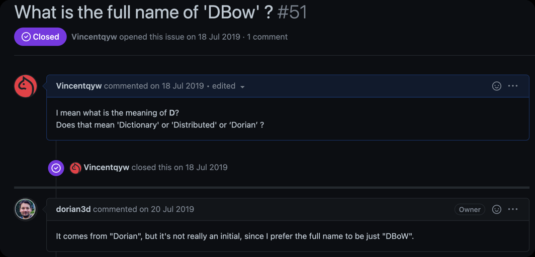
DBoW(2/3): 这是 BoW 的一种 C++ 实现，D 是作者的名字首字母，以下是作者的回复：

BOW参考文献 Video Google: A Text Retrieval Approach to Object Matching in Videos , ICCV 2003.

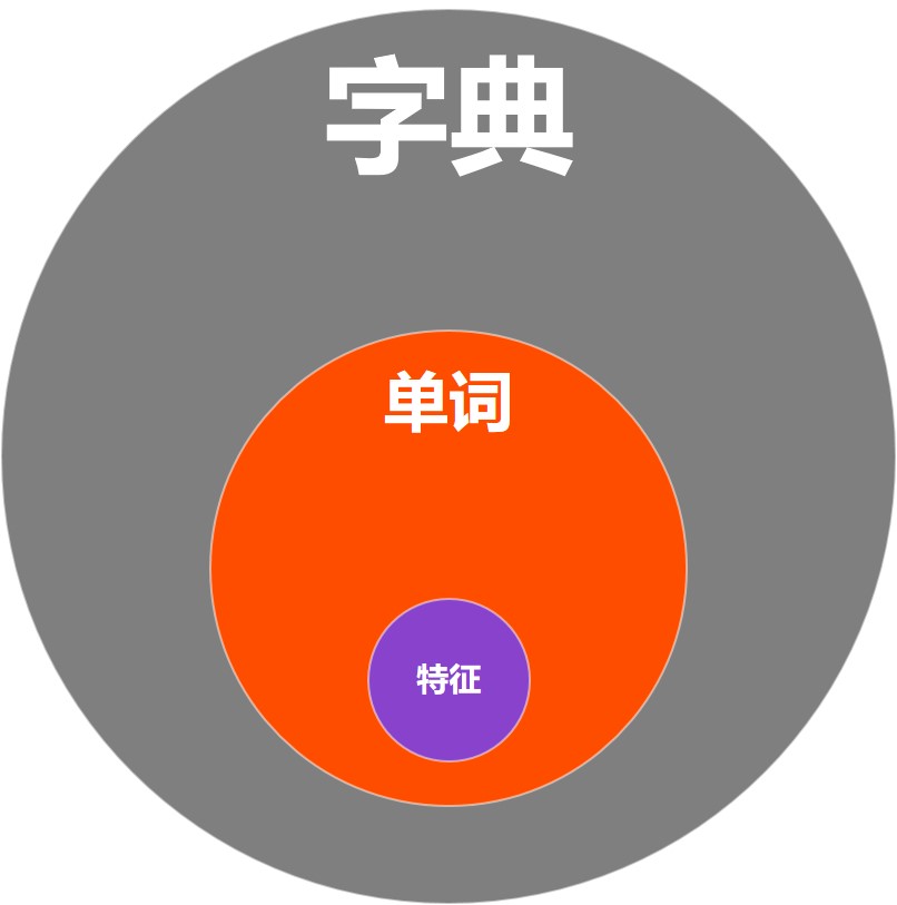
字典/单词/特征

字典是单词的集合，有的地方称为“码书”(codebook)
一个字典里有很多“单词”
一个“单词”底下”挂着” 很多“特征”(可以想象，这些特征因“长得像”所以分在了一个单词下)

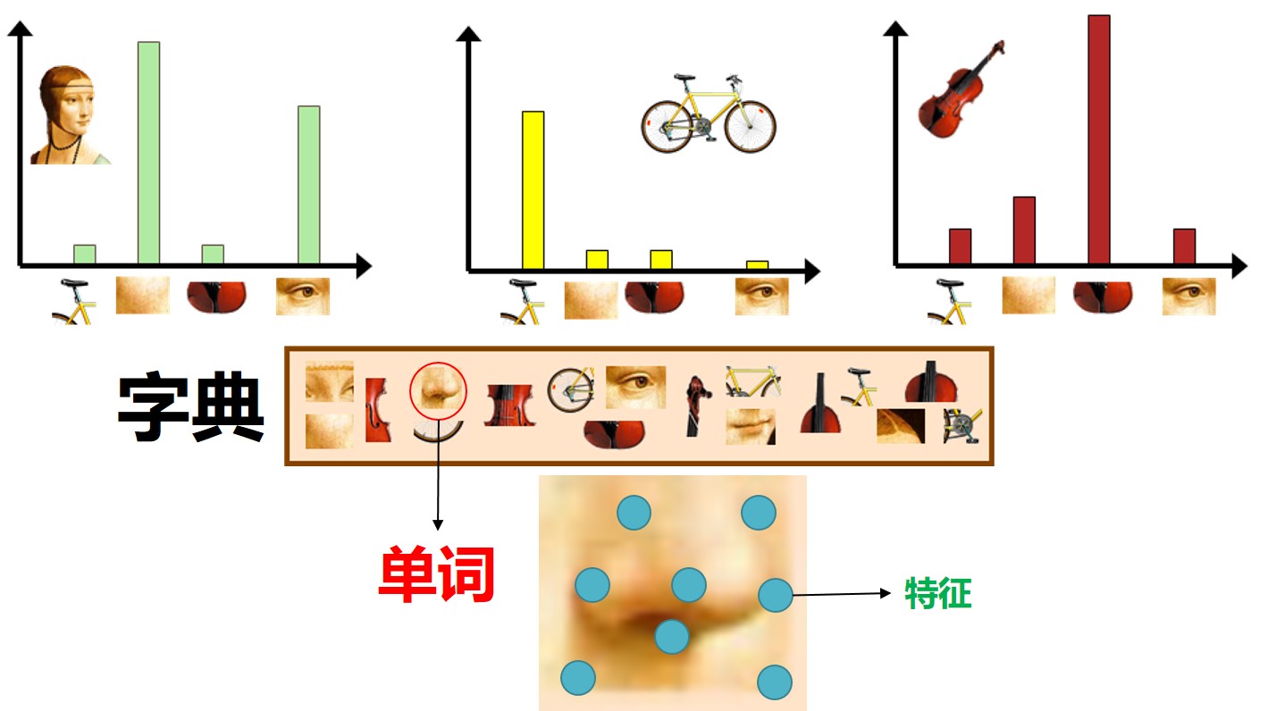
字典，单词与特征的关系可以由下图表示。

如何得到BoW

后续的例子均以SIFT特征为例进行展开介绍。

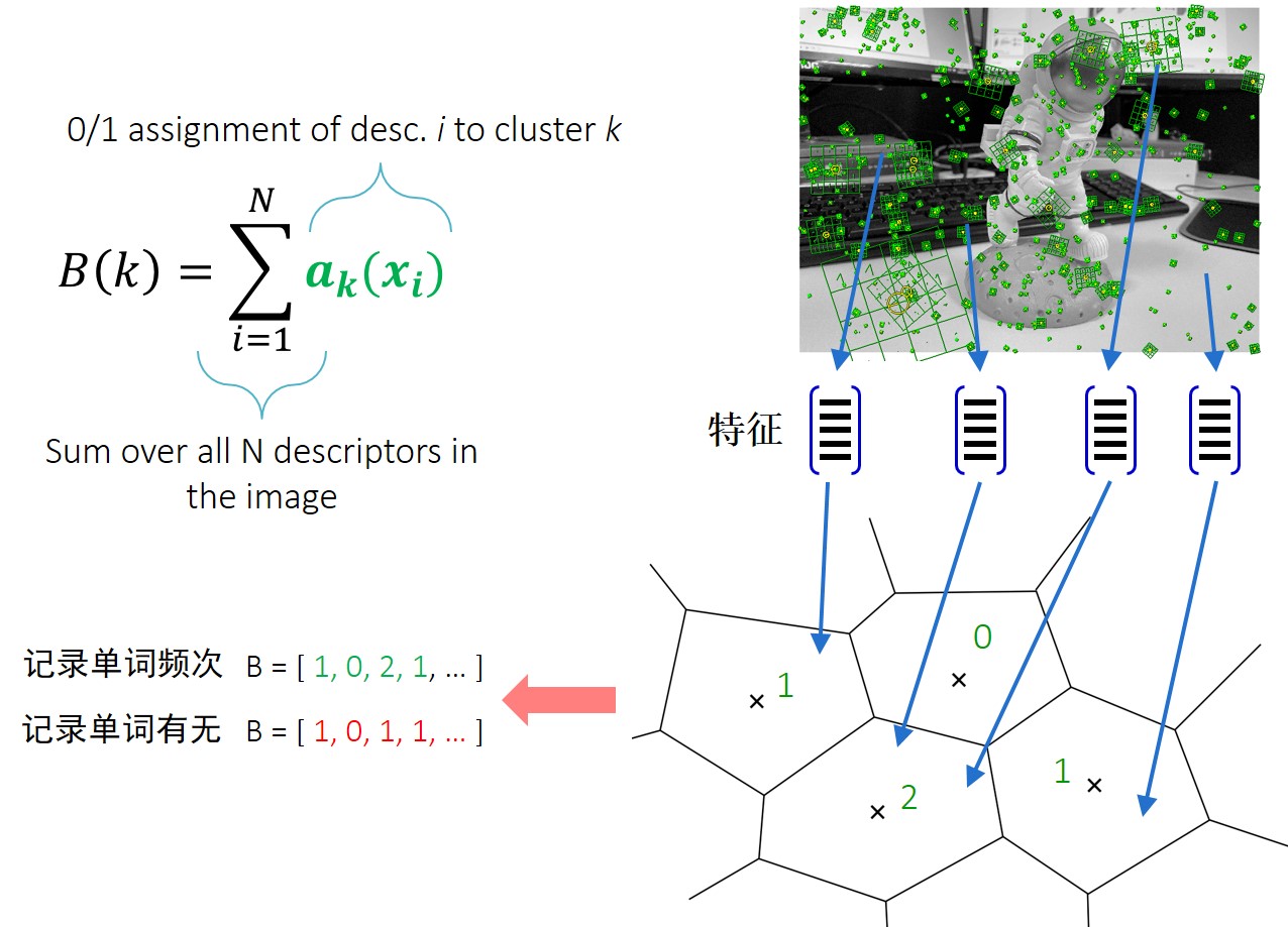
在计算词袋向量之前，我们需要一个训练好的字典（稍后介绍）。对于输入图像，提取SIFT特征，这里的特征指的是特征点及其对应的描述子，计算词袋向量需要的是描述子。我们在字典中查找特征描述子所在的单词，然后在该单词的频次上计数+1，图像上所有特征的描述子找到其对应单词后也就得到了单词出现频次的计数值，我们可以将这个频次称为词袋向量，维度为单词的个数。如上图所示，图像有4个特征，统计特征对应字典种单词出现的频次，这样可以得到该图像的“词袋”向量 $B = [1, 0, 2, 1, ...]$ ，或者我们仅仅保留单词有无出现过，这样可以得到二值化的词袋向量 $B = [1, 0, 1, 1, ...]$ 。

不过，我们这么做的大前提是对每个单词“一视同仁”，但这是有问题的！

试想一下：如果给出一个单词“了”,你能确定是它是来自哪个句子吗？恐怕很难！但是给你一个单词“龍”，你就可能非常快速地找到它的来源。所以“了”和“龍”虽然都是单词，但是它们的重要程度是不一样的。

因此一个成熟的BoW应该具备如下性质：

我们希望，我们构建的字典中单词“了”的权重比单词“龍”的权重要小些！这就需要引入逆向文件频率Inverse document frequency（ $I D F$ ），即构建字典时出现次数多的单词权重小些，出现次数小的单词权重大些。
此外，在分类时，图像中有的单词多有的单词少，此时单词多需要增加权重，单词少要加大权重，这就是词频Term Frequency（ $T F$ ）

对于 $I D F$ ：

I D F_{i} = lo g \frac{n}{n _{i}}

, 其中 $n$ 表示字典中特征总数， $n_{i}$ 表示字典中单词 $i$ 中特征总数， $I D F$ 在训练字典时就可以顺便计算得到。

对于 $T F$ ：

T F_{i} = lo g \frac{m _{i}}{m}

, 其中 $m$ 表示图像上特征总数， $m_{i}$ 表示字典中单词 $i$ 中特征总数，每一张图像的 $T F$ 都不同，需要在查询时进行计算。其实，上面例子中计算的就是词频 $T F$ 。

将使用 $I D F$ 对 $T F$ 加权就可以得到加权后的词袋向量 $η_{i} = T F_{i} \times I D F_{i}$ 。

倒排索引

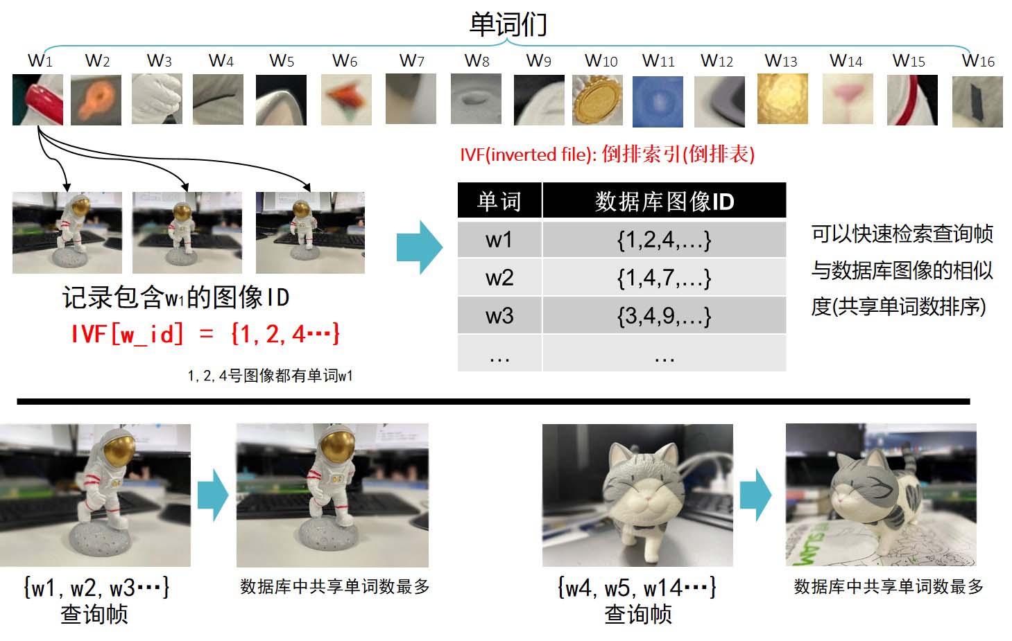
倒排索引记录了单词与图像之间的对应关系，即 $I V F [w_{i d}] = I_{i}$ ，如对于单词 $w_{1}$ ，图像 $1, 2, 4...$ 都有单词 $w_{1}$ 。于是在进行图像检索时，我们可以统计查询图像与数据库图像之间的共享单词的个数，共享单词数量多的数据库图像就是与查询图像“相似”的图像。整个过程中并没有进行图像匹配，仅以统计的方式得到了图像之间的“相似度”，这个过程是非常快速的，因而在SLAM中的重定位/闭环时经常使用。

VLAD

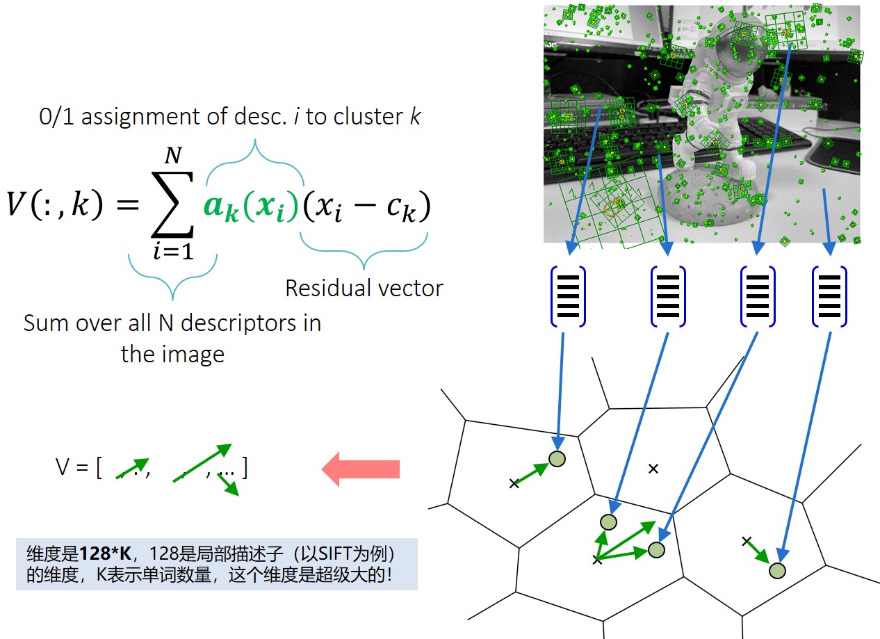
在了解了BoW的计算过程后，VLAD (Vector of Locally Aggregated Descriptor)的计算过程也就非常简单了。VLAD将属于同一个单词的所有特征与单词之间的距离差异（residual vector）累积，得到属于该单词的VLAD向量 $V (:, k)$ 。可以看到，VLAD相较BoW增加了特征与单词之间的距离度量(即保留局部特征与聚类中心的分布差异)。假设单词的数量为 $K$ ，以SIFT为例，每个特征的描述子维度为128，所以VLAD的维度为 $128 \times K$ 。当 $K$ 较大时，VLAD的维度是非常大的，通常后续要进行降维操作。

BoW和VLAD代码实现

废话不多说，直接上代码。本小节使用vlfeat工具箱的Matlab接口对BoW和VLAD进行了实现。

虚拟数据

这里提供了一种使用虚拟数据训练字典得到BoW和VLAD的过程。

close all
% add vlfeat toolbox
run('vlfeat-0.9.21\toolbox\vl_setup');

%% Train a codebook

% trainning data generation
numDatabase    = 10000;
dimLocalDesc   = 128;
X = uint8(floor(255*rand(dimLocalDesc,numDatabase))); % can be computed by vl_sift

% setting params to KMeans
K              = 10; % number of clusters
[centers,assn] = vl_ikmeans(X,K,'verbose');

% build a kd-tree to softassignment
kdtree         = vl_kdtreebuild(single(centers),'verbose');

%% Compute IDF for database
nn_kdtree      = vl_kdtreequery(kdtree, single(centers), single(X));
assignments    = zeros(K,size(X,2));
assignments(sub2ind(size(assignments), nn_kdtree, 1:length(nn))) = 1;
% or: assignments(sub2ind(size(assignments), assn, 1:length(nn))) = 1;

IDF            = log(numDatabase*ones(K,1)./(sum(assignments,2) + 1) );

%% Encode with BOW and VLAD
numofLocalKPs  = 100; % number of keypoints

query          = uint8(floor(255*rand(dimLocalDesc,numofLocalKPs)));  % can be computed by vl_sift
% todo: can be retrieval with vl_ikmeanspush(query,centers) ;
nn             = vl_kdtreequery(kdtree, single(centers), single(query));

% soft assignment
query_assign   = zeros(K,numofLocalKPs);  %only 1 each col
query_assign(sub2ind(size(query_assign), nn, 1:length(nn))) = 1;

% encode with vlad and bow
enc_vlad       = vl_vlad(single(query),single(centers),single(query_assign),'verbose');

enc_bow        = sum(query_assign,2);
numTotalWords  = sum(enc_bow);
TF             = enc_bow / numTotalWords;
enc_bow        = TF .* IDF;

% show
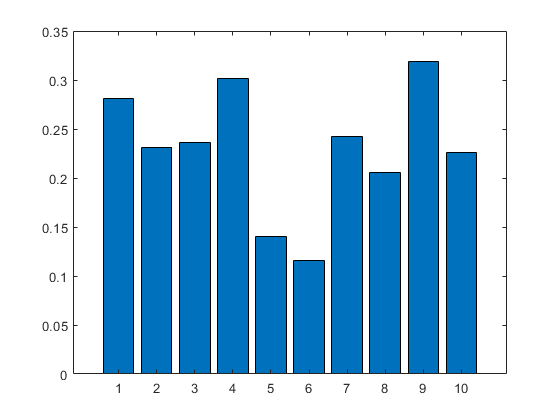
bar(enc_bow);
set(gcf,'color',[1 1 1]);

TF-IDF加权后的BOW向量长这个样子：

真实数据

这里提供了一种使用真实数据训练字典得到BoW和VLAD进行图像相似度比较的实现。

训练

close all;
clear all;
clc

run('vlfeat/toolbox/vl_setup');

%% build kd-tree(KMeans)

base_path       = 'your_image_data_path';

files           = dir(base_path);
database        = [];
already_compute = dir('database.mat');

if numel(already_compute)
    disp(['==> loading database...']);
    load('database.mat');
else
    disp(['==> Extract sift to database...']);
    h = waitbar(0,'Extract sift, please wait');
    for i = 1:numel(files)
        if(files(i).isdir)
            continue;
        end
        image_path = [base_path, files(i).name];
        image      = imread(image_path) ;
        image      = imresize(image,0.5);
        if numel(size(image))== 3
            image      = single(rgb2gray(image)) ;
        else
            image      = single(image);
        end
        [f,d]      = vl_sift(image) ;
        database   = [database,d];
        waitbar(i/numel(files), h,['Extract sift, please wait: ', num2str(i/numel(files)*100), '%' ]);
    end
    close(h);
    save('database.mat','database');
end

numClusters  = 50;
% nleaves    = 10000;
disp(['==> Kmeans running...']);
% [centers, ~] = vl_hikmeans(database, numClusters,nleaves,'verbose');

[centers, associations] = vl_ikmeans(database, numClusters,'verbose');
assign = zeros(numClusters,size(database,2));
assign(sub2ind(size(assign),associations,1:length(associations))) = 1;
IDF    = log(size(database,2) * ones(numClusters,1) ./ (sum(assign,2)+1));

disp(['==> Building KDTree running...']);
kdtree = vl_kdtreebuild(single(centers)); % optional, to accelerate query speed

查询

disp(['==> Query KDTree running...']);
I = imread('Q.png') ;
I = single(rgb2gray(imresize(I,0.8))) ;
[feat_vlad_1,feat_tf_1] = feature_aggregate(I,centers,numClusters);
%[feat_vlad_1,feat_tf_1] = feature_aggregate_kdtree(I,kdtree,centers,numClusters); %optional

I = imread('DB_1.png') ;
I = single(rgb2gray(imresize(I,0.8))) ;
[feat_vlad_2,feat_tf_2] = feature_aggregate(I,centers,numClusters);
%[feat_vlad_2,feat_tf_2] = feature_aggregate_kdtree(I,kdtree,centers,numClusters); %optional

I = imread('DB_2.png') ;
I = single(rgb2gray(imresize(I,0.8))) ;
[feat_vlad_3,feat_tf_3] = feature_aggregate(I,centers,numClusters);
%[feat_vlad_3,feat_tf_3] = feature_aggregate_kdtree(I,kdtree,centers,numClusters); %optional

% weighted by IDF and TF
feat_bow_1 = IDF .* feat_tf_1;
feat_bow_2 = IDF .* feat_tf_2;
feat_bow_3 = IDF .* feat_tf_3;

% higher better
score_vlad1 = feat_vlad_1' * feat_vlad_2;
score_vlad2 = feat_vlad_1' * feat_vlad_3;

% higher better
score_bow1 = computeBowScore(feat_bow_1,feat_bow_2);
score_bow2 = computeBowScore(feat_bow_1,feat_bow_3);

% plot
subplot(311);
bar(feat_bow_1);
set(gca,'xlim',[0,numClusters+1]);
xlabel('cluster index');
subplot(312);
bar(feat_bow_2);
set(gca,'xlim',[0,numClusters+1]);
xlabel('cluster index');
subplot(313);
bar(feat_bow_3);
set(gca,'xlim',[0,numClusters+1]);
xlabel('cluster index');
set(gcf,'color',[1,1,1]);
set(gcf,'pos',[756   301   742   647])

其中feature_aggregate函数输入图像，输出其TF与VLAD编码。笔者提供了两种实现方式，两种方式的区别是后者feature_aggregate_kdtree采用KD-Tree加速了图像特征到单词的查询速度，即编码速度更快（但可能存在精度损失）。

function [vlad,TF] = feature_aggregate(image,centers,numClusters)
    [f,d]  = vl_sift(image) ;
    query  = single(d);
    dim    = size(query,2);
    assign = zeros(numClusters,dim);
    nn     = vl_ikmeanspush(uint8(d) , int32(centers));
    assign(sub2ind(size(assign),nn,1:length(nn))) = 1;
    TF     = sum(assign,2) / sum(assign(:));
    vlad   = vl_vlad(query,single(centers), single(assign),'NormalizeComponents');
end

function [vlad,TF] = feature_aggregate_kdtree(image,kdtree,centers,numClusters)
    [f,d]  = vl_sift(image) ;
    query  = single(d);
    dim    = size(query,2);
    assign = zeros(numClusters,dim);
    nn     = vl_kdtreequery(kdtree,single(centers),single(d));
    assign(sub2ind(size(assign),nn,1:length(nn))) = 1;
    TF     = sum(assign,2) / sum(assign(:));
    vlad   = vl_vlad(query,single(centers), single(assign),'NormalizeComponents');
end

此外，computeBowScore计算词袋向量的相似度（越大越好），实现如下：

function score = computeBowScore(bow1,bow2)
    score = 2 * sum(abs(bow1) + abs(bow2) - abs(bow1- bow2));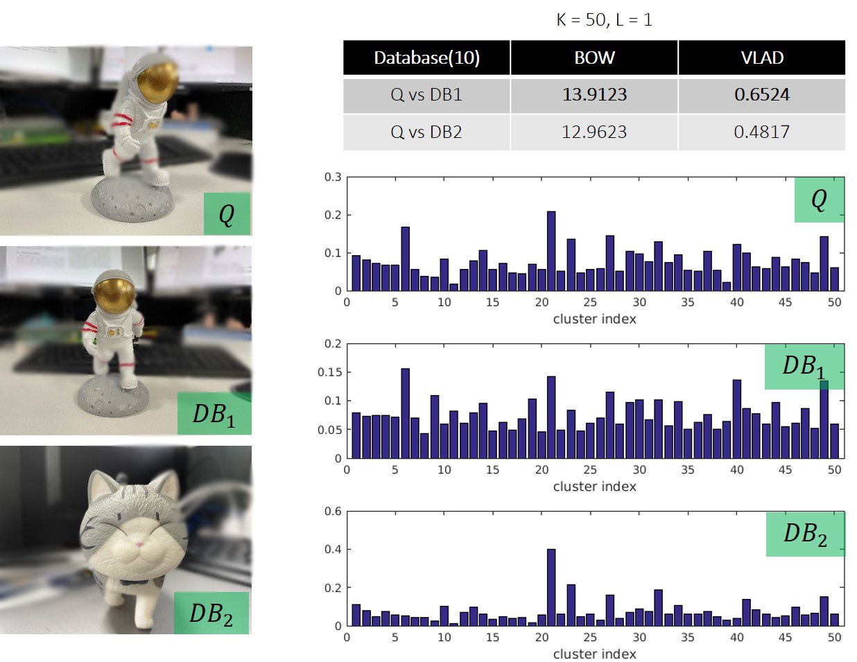
end

下图是查询图与数据库中两张图像的相似度对比。其中 $K = 50, L = 1$ 表示，聚类中心数量为50，这个字典由50个单词组成，层数为1。另外，参与训练字典的图像数量为10。通过主观观察可以明显地看到查询图 $Q$ 与 $D B_{1}$ 相似，与 $D B_{2}$ 不相似；从词袋相似度上可以看到，前者的相似度比后者要高，这说明BoW的有效性。但是二者相似度得分差异并不大，这可能与训练样本数量以及字典层数相关（如何改进？多层+增加训练集合+使用特异性更强的特征点对特征进行描述）。VLAD相似度得分比较位于表格的最后一列，也可以得出 $Q$ 与 $D B_{1}$ 较为相似的结论。

NetVLAD

NetVLAD是对VLAD的进一步改进，使用softmax到单词的对应关系从hard assignment转换成soft assigment（软分配矩阵），遂将VLAD变成了一个学习的过程。

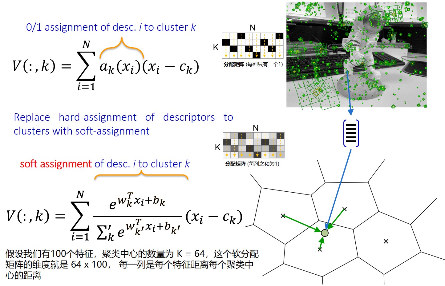
至于这个软分配矩阵，假设我们有100个特征，聚类中心的数量为 K = 64，这个软分配矩阵的维度就是 64 x 100，每一列是每个特征距离每个聚类中心的距离。

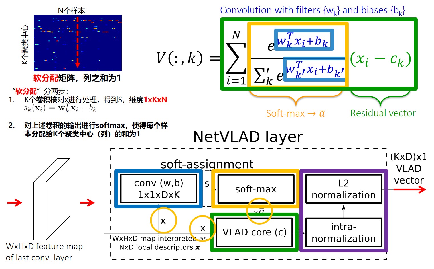
NetVLAD层的处理流程如下：

$x$ 维度是 $1 \times D \times N$ ，其中 $D = 512$ ， $N = H \times W$ ，可以理解成有 $N$ 个 $D$ 维的特征， $N$ 就是特征的个数；
$s$ 就是score，维度： $1 \times K \times N$ ，其中 $K = 64$ ，为“聚类中心” 的数量， $s$ 是将 $x$ 经过卷积得到，这一步在源码中叫做 score_proj（由1D卷积定义）；
$a$ 为软分配矩阵，即通过 $s$ 经过一个softmax得到，维度与 $s$ 相同；
NetVLAD公式中需要计算每个特征与聚类中心的距离diff，它的维度是 $1 \times D \times K \times N$ ，这同样是比较关键的一步：这个diff可以理解成，一共有 $N$ 个特征， $K$ 个聚类中心，所以一共有 $K \times N$ 个距离，这个距离的维度是 $D$ ；
将score与diff相乘，并按照特征维度（最后一维）进行相加，得到desc（即图中的 $V$ ），其维度为 $1 \times D \times K$ ；
将 $V$ 按照dim=1进行归一化（文中称为intra-norm）,即按照特征维度归一化；
将 $V$ 拉成“一条”得到一个维度为 $1 \times (D \times K)$ 的向量，紧接着将这个向量进行L2归一化； 8. 经过第7步之后得到一个 $1 \times (D \times K)$ 的VLAD向量，经过一个“白化”层，对其进行降维，最终得到一个 $1 \times 4096$ 维的向量；

上述处理流程与下面的代码是对应的（可能与上图标记的张量维度有些差异，这一点需要注意）。

推理代码

下面是CVG Hierarchical-Localization项目中公开的netvlad layer的Pytorch实现。

class NetVLADLayer(nn.Module):
    def __init__(self, input_dim=512, K=64, score_bias=False, intranorm=True):
        super().__init__()
        self.score_proj = nn.Conv1d(
            input_dim, K, kernel_size=1, bias=score_bias)
        centers = nn.parameter.Parameter(torch.empty([input_dim, K]))
        nn.init.xavier_uniform_(centers)
        self.register_parameter('centers', centers)
        self.intranorm = intranorm
        self.output_dim = input_dim * K

    def forward(self, x):
        b = x.size(0)
        scores = self.score_proj(x)                                       # DIM: 1xKxN
        scores = F.softmax(scores, dim=1)                                 # DIM: 1xKxN
        diff = (x.unsqueeze(2) - self.centers.unsqueeze(0).unsqueeze(-1)) # DIM: 1xDxKxN
        desc = (scores.unsqueeze(1) * diff).sum(dim=-1)                   # DIM: 1xDxK
        if self.intranorm:
            # From the official MATLAB implementation.
            desc = F.normalize(desc, dim=1)                               # DIM: 1xDxK
        desc = desc.view(b, -1)
        desc = F.normalize(desc, dim=1)                                   # DIM: 1x(DxK)
        return desc

后续的白化层whiten layer通过一个全连接层来定义：

self.whiten = nn.Linear(self.netvlad.output_dim, 4096)   # IN_DIM: 1x(DxK), OUT_DIM: 1x4096

将主干网络与NetVLAD层串起来得到forward，代码如下:

def _forward(self, data):
    image = data['image']
    assert image.shape[1] == 3
    assert image.min() >= -EPS and image.max() <= 1 + EPS
    image = torch.clamp(image * 255, 0.0, 255.0)  # Input should be 0-255.
    mean  = self.preprocess['mean']
    std   = self.preprocess['std']
    image = image - image.new_tensor(mean).view(1, -1, 1, 1)
    image = image / image.new_tensor(std).view(1, -1, 1, 1)

    # Feature extraction.
    descriptors = self.backbone(image)
    b, c, _, _  = descriptors.size()
    descriptors = descriptors.view(b, c, -1) # DIM: bx512xN, N = H'x w'

    # NetVLAD layer.
    descriptors = F.normalize(descriptors, dim=1)  # Pre-normalization.
    desc = self.netvlad(descriptors)     # DIM: bx(DxK)

    # Whiten if needed.
    if hasattr(self, 'whiten'):
        desc = self.whiten(desc)
        desc = F.normalize(desc, dim=1)  # Final L2 normalization, DIM: bx4096

    return {
        'global_descriptor': desc
    }

Loss项

训练样本来自Google Street View Time Machine(谷歌街景时光机)。

给定查询帧, 街景数据会提供给我们百分百错误的候选帧 (geographically far from the query)

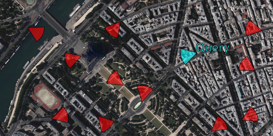
给定查询帧, 街景数据会提供给我们可能的候选帧 (geographically close to the query)

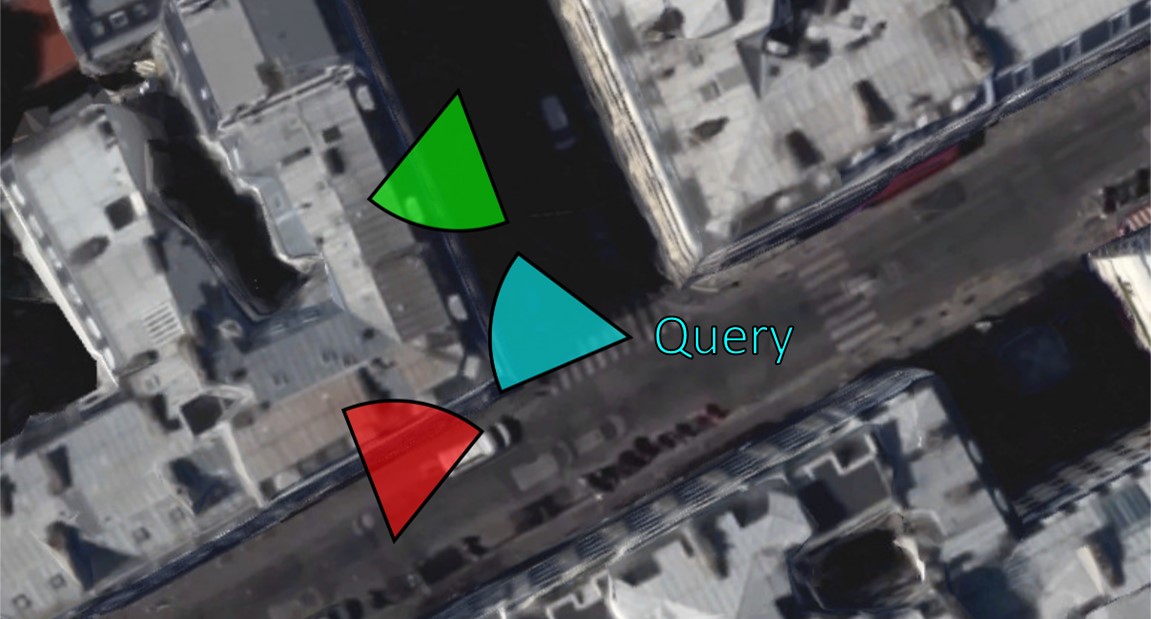
NetVLAD的loss采用了triplet-loss。

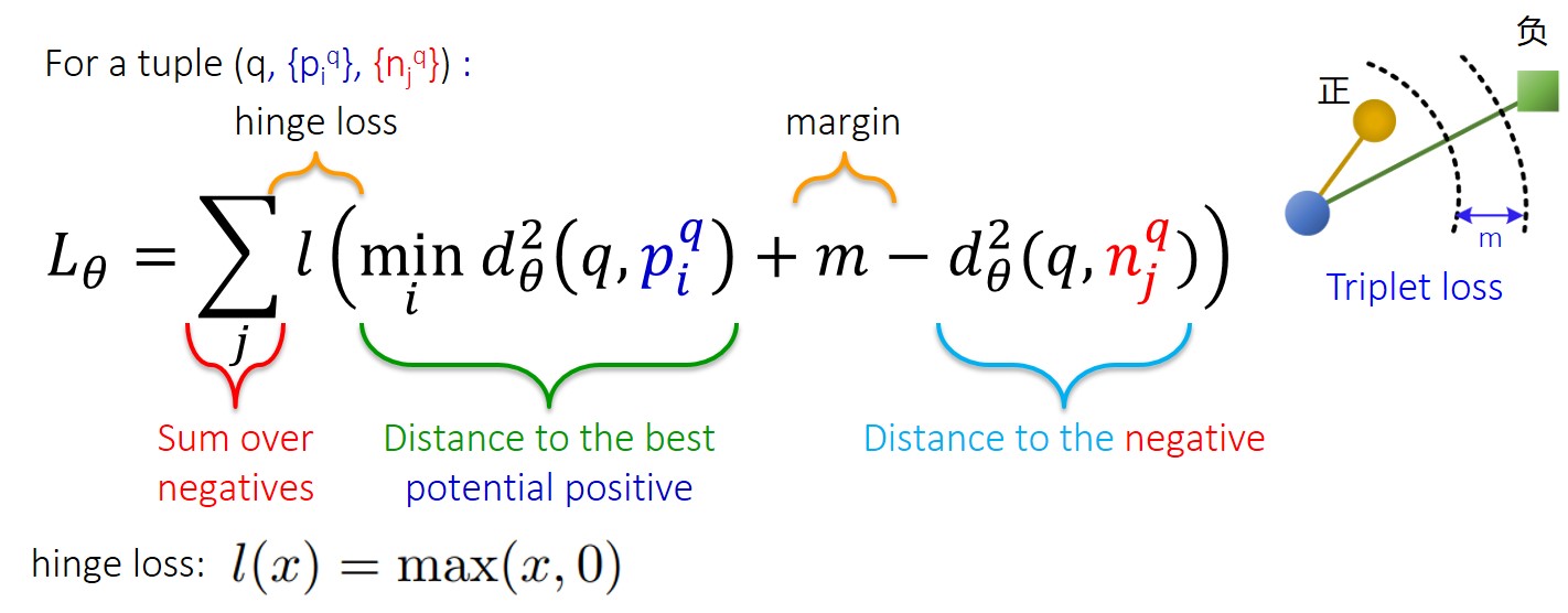
目标：学习一个网络使得查询帧与正例之间的最小距离 $d_{1}$ 要小于查询帧与所有负例之间的距离 $d_{2}$ 。但仅仅 $d_{2} - d_{1} > 0$ 并不够，还要求 $d_{2}$ 比 $d_{1}$ 大上一段距离，这个距离为上式中的 $m$ 。所以，当 $d_2- d_1 < m$ 时，这说明网络还不足以区分正、负例，我们要惩罚这种现象（即，此时的 $l (x) = x$ ）;对应的，当 $d_{2} - d_{1} \geq m$ 时，网络可以区分正、负例，此时的惩罚为0。

参考

vlfeat: Integer k-means: https://www.vlfeat.org/overview/ikm.html
vlfeat: Hierarchical Integer k-means: https://www.vlfeat.org/overview/hikm.html
R Arandjelovic et.al. All about VLAD, 2013
ETH Zurich, Computer Vision and Geometry Lab(CVG), NetVLAD code, 2021
NetVLAD: CNN architecture for weakly supervised place recognition, [Homepage] , [Paper on arXiv] [Presentation (54 MB)], CVPR 2016