Matlab Deep Learning学习笔记

最近对深度学习尤其着迷，是时候用万能的Matlab去践行我的DL学习之路了。之所以用Matlab，是因为Matlab真的太强大了！自从大学开始我就一直用这个神奇的软件，算是最熟悉的编程工具。加上最近mathworks公司一大波大佬的不懈努力，在今年下半年发行的R2017b版本中又加入了诸多新颖的特性，尤其在DL方面，可以发现：仅仅几条简单的代码，就能够实现复杂的功能。基于以上，我在本文列举了几个在Matlab上学习Deep Learning的例子：1. 手写字符识别；2. 搭建网络对CIFAR10分类；3.搭建一个Resnet。务必保证主机已经安装Matlab 2017a及以上。

手写字符识别

利用CNN做数字分类实验。

接下来的实验会阐明如何进行： - 加载图像数据 - 设计网络结构 - 设置网络训练参数 - 训练网络 - 预测新数据的类别

加载图像数据

digitDatasetPath = fullfile(matlabroot,'toolbox','nnet','nndemos',...
    'nndatasets','DigitDataset');
% imageDatastore函数 能够通过文件夹名自动地把数据存储成ImageDatastore 对象
digitData = imageDatastore(digitDatasetPath,...
    'IncludeSubfolders',true,'LabelSource','foldernames');

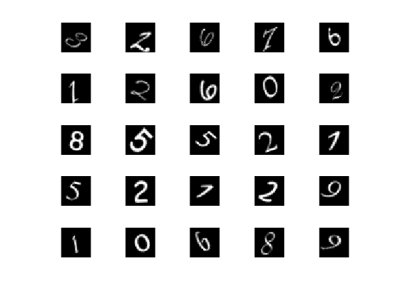
% Display some of the images in the datastore.
figure;
perm = randperm(10000,25);
for i = 1:25
    subplot(5,5,i);
    imshow(digitData.Files{perm(i)});
end

以下是手写字符的部分数据：

创建训练集与验证集

trainNumFiles = 750;
[trainDigitData,valDigitData] = splitEachLabel(digitData,750,'randomize');
% 每类有1000个，选择其中的750类作为训练集，剩下的作为验证集；此处750可以换成一个比例：75%

注意Matlab里面支持的层的类型，包括：CLICK THIS LINK。如下所示：

Epoch

Iteration

Layer Type

Function

Image input layer

imageInputLayer

Sequence input layer

sequenceInputLayer

2-D convolutional layer

convolution2dLayer

2-D transposed convolutional layer

transposedConv2dLayer

Fully connected layer

fullyConnectedLayer

Long short-term memory (LSTM) layer

LSTMLayer

Rectified linear unit (ReLU) layer

reluLayer

Leaky rectified linear unit (ReLU) layer

leakyReluLayer

Clipped rectified linear unit (ReLU) layer

clippedReluLayer

Batch normalization layer

batchNormalizationLayer

Channel-wise local response normalization (LRN) layer

crossChannelNormalizationLayer

Dropout layer

dropoutLayer

Addition layer

additionLayer

Depth concatenation layer

depthConcatenationLayer

Average pooling layer

averagePooling2dLayer

Max pooling layer

maxPooling2dLayer

Max unpooling layer

maxUnpooling2dLayer

Softmax layer

softmaxLayer

Classification layer

classificationLayer

Regression layer

regressionLayer

创建自己的网络结构

%% Define Network Architecture
% Define the convolutional neural network architecture.
layers =
    [
    imageInputLayer([28 28 1])
    convolution2dLayer(3,16,'Padding',1)
    batchNormalizationLayer()
    reluLayer()
    maxPooling2dLayer(2,'Stride',2)

    convolution2dLayer(3,32,'Padding',1)
    batchNormalizationLayer()
    reluLayer()

    maxPooling2dLayer(2,'Stride',2)

    convolution2dLayer(3,64,'Padding',1)
    batchNormalizationLayer()
    reluLayer()

    fullyConnectedLayer(10)
    softmaxLayer()
    classificationLayer()
    ];

以下就是该网络结构及参数设置：

Image Input             28x28x1 images with 'zerocenter' normalization
Convolution             16 3x3 convolutions with stride [1  1] and padding [1  1  1  1]
Batch Normalization     Batch normalization
ReLU                    ReLU
Max Pooling             2x2 max pooling with stride [2  2] and padding [0  0  0  0]
Convolution             32 3x3 convolutions with stride [1  1] and padding [1  1  1  1]
Batch Normalization     Batch normalization
ReLU                    ReLU
Max Pooling             2x2 max pooling with stride [2  2] and padding [0  0  0  0]
Convolution             64 3x3 convolutions with stride [1  1] and padding [1  1  1  1]
Batch Normalization     Batch normalization
ReLU                    ReLU
Fully Connected         10 fully connected layer
Softmax                 softmax
Classification Output   crossentropyex

网络训练参数设计

 options = trainingOptions('sgdm',...
'MaxEpochs',3, ...                 % 训练最大轮回
'ValidationData',valDigitData,...  % 验证集
'ValidationFrequency',30,...
'Verbose',false,...
'Plots','training-progress');

开始训练

net = trainNetwork(trainDigitData,layers,options);

测试新的数据

predictedLabels = classify(net,valDigitData);
valLabels = valDigitData.Labels;
accuracy = sum(predictedLabels == valLabels)/numel(valLabels)

查看某层参数

例如查看第2层的weight参数，输入以下命令：

montage(imresize(mat2gray(net.Layers(2).Weights),[128 128]));
set(gcf,'color',[1 1 1]);
frame=getframe(gcf); % get the frame
image=frame.cdata;
[image,map]     =  rgb2ind(image,256);
imwrite(image,map,'weight-layer2.png');

图像如下所示：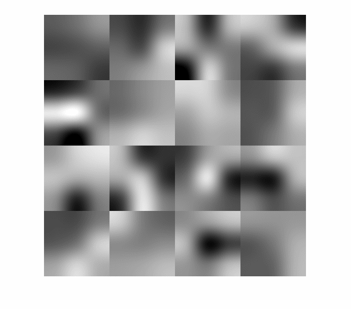

再看一下第10层的参数：

[~,~,iter,~]=size(net.Layers(10).Weights);
name='weight.gif';
dt=0.4;
for i=1:iter
	montage(imresize(mat2gray(net.Layers(10).Weights(:,:,i,:)),[128 128]));
    set(gcf,'color',[1 1 1]); %变白
	title(['Layer(10), Channel: ',num2str(i)]);
	axis normal
	truesize
	%Creat GIF
	frame(i)=getframe(gcf); % get the frame
	image=frame(i).cdata;
	[image,map]     =  rgb2ind(image,256);
	if i==1
		 imwrite(image,map,name,'gif');
	else
		 imwrite(image,map,name,'gif','WriteMode','append','DelayTime',dt);
    end
end

搭建网络对CIFAR10分类

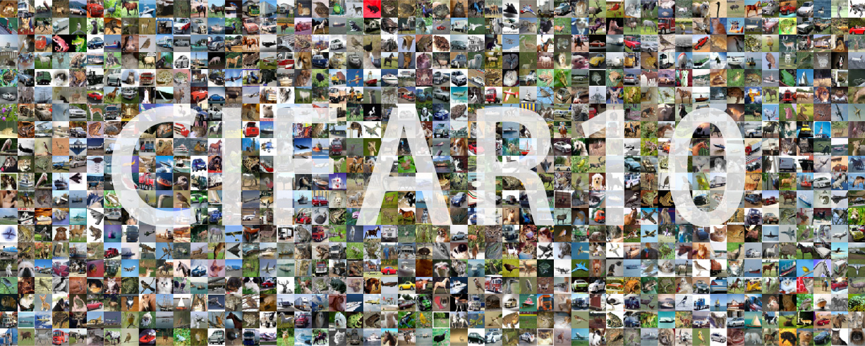
CIFAR10和CIFAR100是80 million tiny images的子集，是由Geoffrey Hinton的弟子们Alex Krizhevsky和Vinod Nair共同采集。

CIFAR10

CIFAR10由60000张32*32的彩色图像组成，一种分成10类，平均每类图像6000张。共有50000张训练图像，10000张测试图像。这个数据集被分成了5个分支，其中每个分支10000张。测试集包含每类中随机选择的1000张图像。训练集就是剩下的那些图像。

对于每个分支的数据的大小是：10000*3072；其中3072=32*32*3。数据以行优先的顺序存储，所以前1024个数据是r通道的数据，接下来的1024个数据是g通道的数据，最后1024个数据是b通道的。假如原始的数据是data，我们想要将其重新排列成我们需要的数据。首先对其进行转置，然后再用reshape函数对图像重组（可选：最后将图像前两维互换（转置），之所以这么做，可以更好的可视化）。

XBatch = data';
XBatch = reshape(XBatch, 32,32,3,[]);
XBatch = permute(XBatch, [2 1 3 4]);

以下是cifar10的部分数据。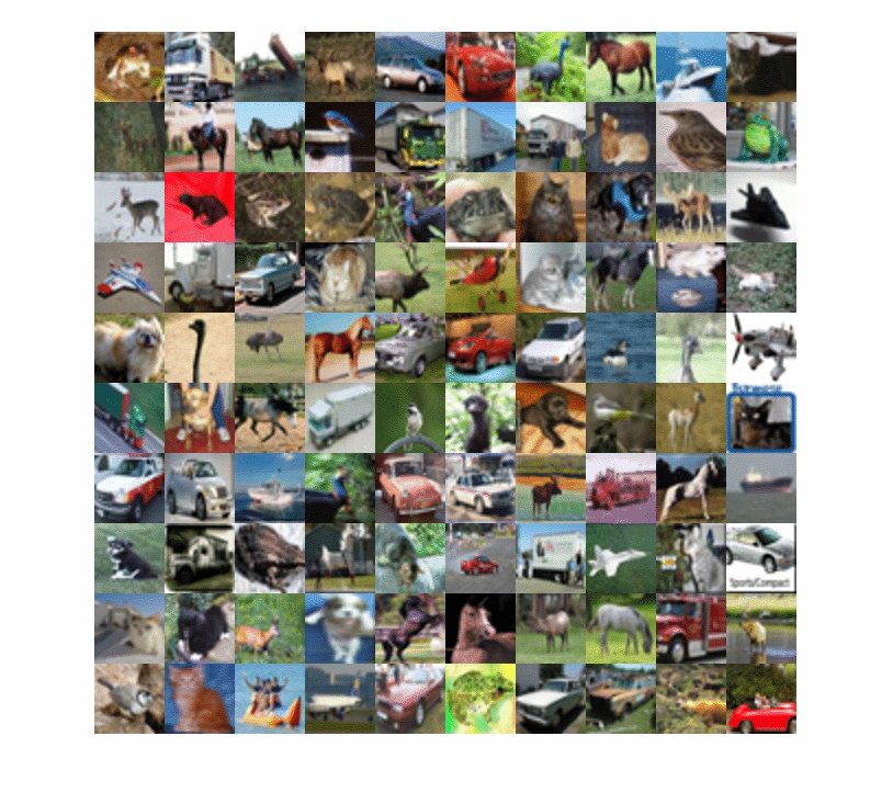共有10类，包括：airplane，automobile，bird，cat，deer，dog，frog，horse，ship，truck。

Just run it

接下来我们就开始运行以下代码，来训练我们的网络。闲话少说，我把代码放在了Github，欢迎 $s t a r$ 。

1   'imageinput'    Image Input         	28x28x1 images with 'zerocenter' normalization
2   'conv_1'        Convolution         	16 3x3x1 convolutions with stride [1  1] and padding [1  1  1  1]
3   'batchnorm_1'   Batch Normalization 	Batch normalization with 16 channels
4   'relu_1'        ReLU               		ReLU
5   'maxpool_1'     Max Pooling         	2x2 max pooling with stride [2  2] and padding [0 0  0  0]
6   'conv_2'        Convolution         	32 3x3x16 convolutions with stride [1  1] and padding [1  1  1  1]
7   'batchnorm_2'   Batch Normalization 	Batch normalization with 32 channels
8   'relu_2'        ReLU                	ReLU
9   'maxpool_2'     Max Pooling         	2x2 max pooling with stride [2  2] and padding [0  0  0 0]
10   'conv_3'       Convolution         	64 3x3x32 convolutions with stride [1  1] and padding [1 1  1  1]
11   'batchnorm_3'  Batch Normalization 	Batch normalization with 64 channels
12   'relu_3'       ReLU			ReLU
13   'fc'           Fully Connected		10 fully connected layer
14   'softmax'      Softmax			softmax
15   'classoutput'  Classification Output	crossentropyex with '0', '1', and 8 other classes

以下是训练过程输出：

Epoch

Iteration

Time Elapsed (seconds)

Mini-batch Loss

Mini-batch Accuracy

Base Learning Rate

0.06

2.3026

8.59%

0.0020

1.27

2.3026

14.06%

0.0020

100

2.52

2.3024

7.81%

0.0020

150

3.73

2.2999

20.31%

0.0020

200

5.01

2.2740

15.63%

0.0020

250

6.28

2.1194

21.09%

0.0020

300

7.58

1.9100

23.44%

0.0020

350

8.86

1.8892

28.13%

0.0020

400

10.08

1.7490

29.69%

0.0020

450

11.32

1.8377

31.25%

0.0020

500

12.57

1.6073

39.84%

0.0020

…

7650

407.74

0.2858

93.75%

2.00e-05

7700

409.06

0.3127

89.84%

2.00e-05

7750

410.38

0.3254

87.50%

2.00e-05

7800

411.64

0.2456

92.19%

2.00e-05

最后测试我们的模型的性能，accuracy=76%左右。但是训练时，我们的batch-accuracy已经达到了90%以上，说明我们的模型过拟合了。显然这不是我们想要的结果，进一步的调参将会在此补充。

可视化某层的参数

% Extract the first convolutional layer weights
w = cifar10Net.Layers(2).Weights;

% rescale and resize the weights for better visualization
w = mat2gray(w);
w = imresize(w, [100 100]);

figure
montage(w)
name='cifar10-weight-layer2';
set(gcf,'color',[1 1 1]);
frame=getframe(gcf); % get the frame
image=frame.cdata;
[image,map]     =  rgb2ind(image,256);
imwrite(image,map,[name,'.png']);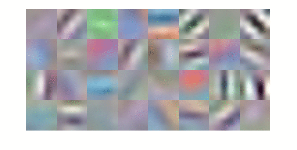

搭建一个Resnet

接下来，为了验证下这个DL工具包的强大之处，我打算纯手工建一个Resnet。为方便起见，我搭了一个Resnet34（更深的网络敬请期待吧）。这里是它的prototxt，我们可以用网络可视化工具进行查看resnet34的结构。以下是Resnet34的一部分（太长了没有截下全部视图）。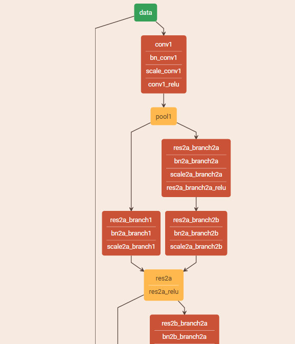

定义每一层与连接层

以从pool1到res2a为例子建立网络。

layers_example=[
    % pool1 - res2a
    maxPooling2dLayer(3, 'Stride', 2,'Name','pool1');
    %  branch2a
    convolution2dLayer(3,64,'Stride', 1,'Padding', 1,'Name','res2a_branch2a')
    batchNormalizationLayer('Name','bn2a_branch2a')
    reluLayer('Name','res2a_branch2a_relu')

    %  branch2b
    convolution2dLayer(3,64,'Stride', 1,'Padding', 1,'Name','res2a_branch2b')
    batchNormalizationLayer('Name','bn2a_branch2b')

    % add together
    additionLayer(2,'Name','res2a')
    reluLayer('Name','res2a_relu')
];

上述过程仅仅完成了网络的一个小分支，记下来要完成res2a_branch1这部分的连接。这时候要用到DAG的一些方法。通过添加新层同时建立新的连接即可，方式如下。

lgraph = layerGraph(layers_example);
figure
plot(lgraph)

%% add some connections (shortcut)
layers_2a=[
    convolution2dLayer(1,64,'Stride', 1,'Padding', 0,'Name','res2a_branch1')
    batchNormalizationLayer('Name','bn2a_branch1')
];
lgraph = addLayers(lgraph,layers_2a);
lgraph = connectLayers(lgraph,'pool1','res2a_branch1');
lgraph = connectLayers(lgraph,'bn2a_branch1','res2a/in2');
% show net
plot(lgraph)

其他部分的构建同上，经过一系列重复的工作，我们可以构建出这个不太深的Resnet34，全部代码见我的Github。

一些基本问题

参数的基本格式

H e i g h t \times W i d t h \times (# C hann e l s) \times (# F i l t er s)

SGD是什么？可以参见好友写的一篇博文。
什么是epoch？模型训练的时候一般采用stochastic gradient descent（SGD），一次迭代选取一个batch进行update。一个epoch的意思就是迭代次数*batch的数目和训练数据的个数一样，就是一个epoch。
为什么要是用BN？ Batch normalization layers normalize the activations and gradients propagating through a network, making network training an easier optimization problem. Use batch normalization layers between convolutional layers and nonlinearities, such as ReLU layers, to speed up network training and reduce the sensitivity to network initialization.
RELU的作用？ Max-Pooling Layer Convolutional layers (with activation functions) are sometimes followed by a down-sampling operation that reduces the spatial size of the feature map and removes redundant spatial information. Down-sampling makes it possible to increase the number of filters in deeper convolutional layers without increasing the required amount of computation per layer. One way of down-sampling is using a max pooling. The max pooling layer returns the maximum values of rectangular regions of inputs.
Resnet中scale层是如何定义的？有什么用途？
Resnet中为何残差 $F (x)$ 比 $H (x)$ 好学？
add more